卷积神经网络
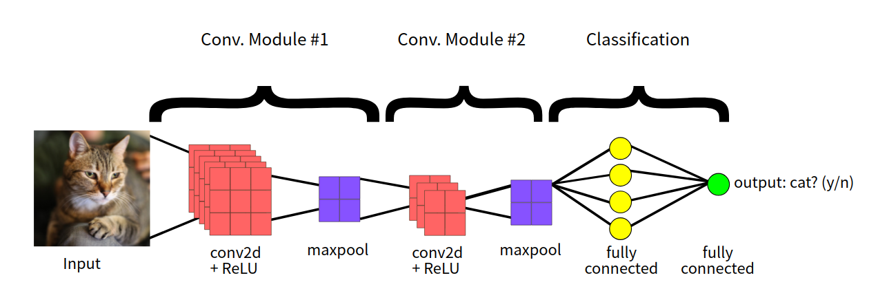
卷积神经网络主要包括 3 层,即:卷积层、池化层以及全连接层。本文讲分别细致介绍这三层的作用和计算来复习一下卷积神经网络。本文采用简单的 LeNet 来讨论这些问题,模型的结构如下。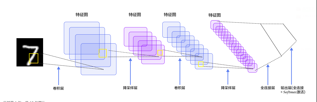
卷积层
卷积层的功能是特征提取。我们先设定下面的符号:
- H:图片高度;
- W:图片宽度;
- D:原始图片通道数,也是卷积核个数;
- F:卷积核高宽大小;
- P:图像边扩充大小;
- S:滑动步长
- K:卷积核的个数
在卷积操作中卷积核是可学习的参数,每层卷积的参数大小为 D×F×F×K。这样看来卷积层的参数还是比较少的,主要原因是采用了两个重要的特性:局部连接和权值共享。
- 局部连接
从神经网络连接结构的角度,CNN 的底层与隐藏不再是全连接,而是局部区域的成块连接: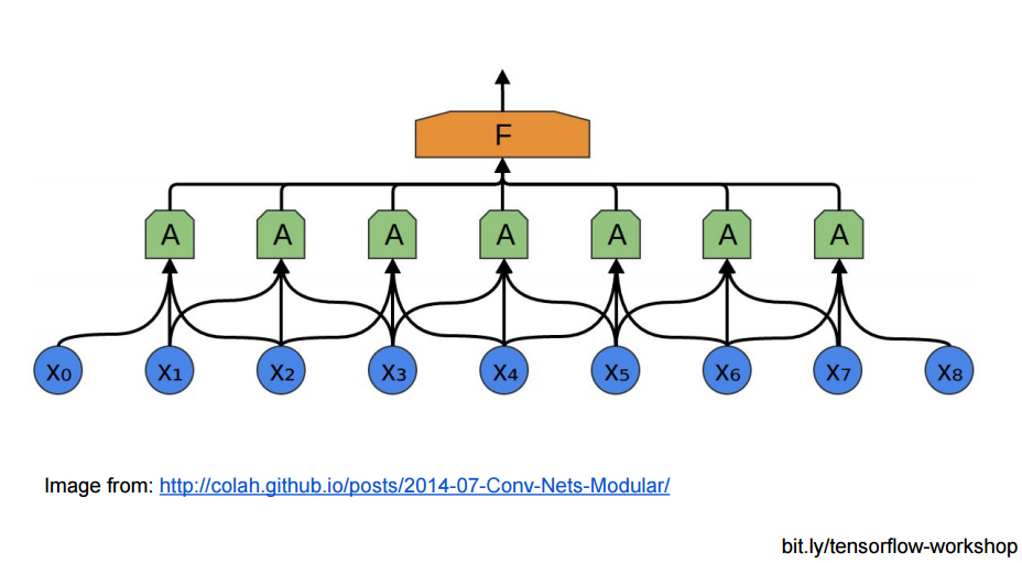
成块连接后,那些小块,还能在上层聚集成更大的块: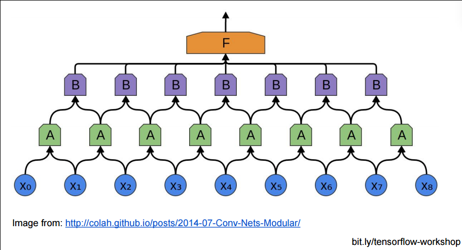
- 权值共享
给一张输入图片,用一个 filter 去扫这张图,filter 里面的数就叫权重,这张图每个位置就是被同样的 filter 扫的,所以权重是一样的,也就是共享。
池化层
如果用上面的方法堆砌 CNN 网络,隐藏层的参数还是太多了,不是吗?每个相邻块都要在上层生成一个大的块。所以有时我们为了减少参数复杂度,不严格把相邻的块都至少聚合成一个上层块,我们可以把下层块分一些区域,在这些区域中聚合: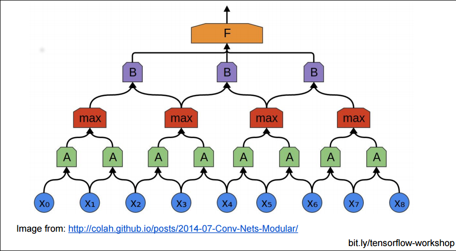
所以池化层的功能主要是对输入的特征图进行压缩,一方面使特征图变小,简化网络计算复杂度;另一方面进行特征压缩,提取主要特征。
最常见的池化操作为平均池化 mean pooling 和最大池化 max pooling:
- 平均池化:计算图像区域的平均值作为该区域池化后的值。
- 最大池化:选图像区域的最大值作为该区域池化后的值。
3D 的卷积和池化如图所示: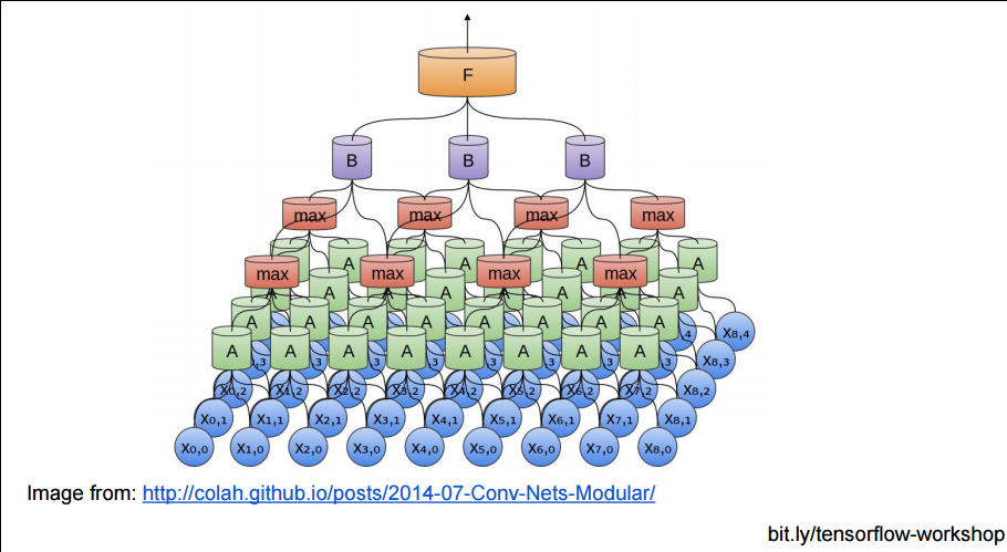
全连接层
卷积取的是局部特征,全连接就是把以前的局部特征重新通过权值矩阵组装成完整的图,将输出值送给分类器(如 softmax 分类器)。
LeNet
第一层,卷积层
输入图像的大小 32x32x1, 卷积核尺寸为 5x5,深度为 6,不使用全 0 填充,步长为 1。所以这一层的输出:28x28x6,卷积层共有 5x5x1x6+6=156 个参数。
第二层,池化层
这一层的输入为第一层的输出,是一个 28x28x6 的节点矩阵。本层采用的过滤器大小为 2x2,长和宽的步长均为 2,所以本层的输出矩阵大小为 14x14x6。
第三层,卷积层
本层的输入矩阵大小为 14x14x6,使用的过滤器大小为 5x5,深度为 16. 本层不使用全 0 填充,步长为 1。本层的输出矩阵大小为 10x10x16。本层有 5x5x6x16+16=2416 个参数。
第四层,池化层
本层的输入矩阵大小 10x10x16。本层采用的过滤器大小为 2x2,长和宽的步长均为 2,所以本层的输出矩阵大小为 5x5x16。
第五层,全连接层
本层的输入矩阵大小为 5x5x16,在 LeNet-5 论文中将这一层成为卷积层,但是因为过滤器的大小就是 5x5,所以和全连接层没有区别。如果将 5x5x16 矩阵中的节点拉成一个向量,那么这一层和全连接层就一样了。本层的输出节点个数为 120,总共有 5x5x16x120+120=48120 个参数。
第六层,全连接层
本层的输入节点个数为 120 个,输出节点个数为 84 个,总共参数为 120x84+84=10164 个。
第七层,全连接层
本层的输入节点个数为 84 个,输出节点个数为 10 个,总共参数为 84x10+10=850
一些有用的代码
在 NoteBook 里面显示训练用到的图片
1 | %matplotlib inline |
主要使用 matplotlib 画一个 4x4 的图,代码效果如下:
Keras 图像增强
通过对现有图像执行随机变换来人为地增加训练样例的多样性和数量,以创建一组新变体。当原始训练数据集相对较小时,数据增加特别有用。
1 | from tensorflow.keras.preprocessing.image import ImageDataGenerator |
ImageDataGenerator的一些参数介绍:
- rotation_range is a value in degrees (0–180), a range within which to randomly rotate pictures.
- width_shift and height_shift are ranges (as a fraction of total width or height) within which to randomly translate pictures vertically or horizontally.
- shear_range is for randomly applying shearing transformations.
- zoom_range is for randomly zooming inside pictures.
- horizontal_flip is for randomly flipping half of the images horizontally. This is relevant when there are no assumptions of horizontal assymmetry (e.g. real-world pictures).
- fill_mode is the strategy used for filling in newly created pixels, which can appear after a rotation or a width/height shift.

可视化中间层
1 | import numpy as np |

可以看出,从浅到深模型学习到的特征越来越抽象,图像的原始像素的信息越来越少,但是关于图像类别的信息越来越精细。
Loss 和 Acc 可视化
1 | # Retrieve a list of accuracy results on training and test data |

上图表示模型过拟合了,简单来说就是训练集和验证集上模型表现不一致。主要原因的数据集太小,一些示例太少,导致模型学习到的知识推广不到新的数据集上,即当模型开始用不相关的特征进行预测的时候就会发生过拟合。例如,如果你作为人类,只能看到三个伐木工人的图像,以及三个水手人的图像,其中唯一一个戴帽子的人是伐木工人,你可能会开始认为戴着帽子是一名伐木工人而不是水手的标志。然后你会做一个非常差的伐木工人 / 水手分类器。